Peak Shaving with Edge Device Control
This tutorial walks you through setting up automated peak shaving for a commercial building. By the end, your edge device will continuously monitor grid power and automatically shed or curtail loads when consumption approaches the peak limit — saving you money on demand charges every month.
What you will build
A complete peak shaving loop:
Continuous cycle every 10–60 seconds
The edge device runs a Conductor — a two-point (bang-bang) controller with hysteresis — that evaluates grid power against the current peak limit and orchestrates load controllers to keep consumption below the threshold.
Requirements
- Edge device registered to the site (Base Mini, Base Safe, or Base Virtual)
- Energy metering module subscription
- Technical systems module subscription
- Grid power meter connected to the edge device (Modbus, MQTT, OBiX, or other supported protocol) reporting total site consumption in kW
- At least one controllable load connected to the same edge device (battery inverter, HVAC, lighting, etc.)
Architecture overview
The system has three layers, each with a distinct role:
| Layer | Component | Responsibility |
|---|---|---|
| Cloud | Peak Shaving Calculator (AI Cloud Meter) | Calculates optimal hourly kW limits from historical data and tariff rules |
| Edge | Peak Shaving Conductor (Bench node) | Real-time control loop — reads grid meter, compares to limit, orchestrates loads |
| Field | Controllers, inverters, VFDs | Physical equipment that responds to setpoint commands |
Why edge, not cloud?
Peak shaving decisions must happen in seconds, not minutes. The conductor runs locally on the edge device with direct access to the grid meter and control datapoints — no round-trip to the cloud. The cloud provides the strategic limit (what to target), the edge provides the tactical response (how to stay under it).
Step 1 — Set up the energy metering technical system
The grid power meter is the conductor's primary input. It must be a connected technical system with a datapoint that reports total site consumption in kW.
Create the technical system
- Open your site and navigate to Technical Systems
- Click New Technical System
- Configure:
- Name — e.g., "Main Grid Meter" or "Utility Incoming Feed"
- Type —
EnergyorMetering
- Save
Connect the grid meter datapoint
The edge device must have a technical connection (Modbus TCP, MQTT, OBiX, etc.) to the physical meter. Within that connection, configure a datapoint for grid power:
| Field | Value |
|---|---|
| Name | Grid Power (kW) |
| Access type | READ |
| Collection type | consumption or meter |
| Flow direction | grid-import |
| Value unit | kW |
| Analytics interval | The meter's reporting interval (e.g. 1000 ms for real-time, 60000 ms for 1-minute) |
If your meter reports in watts, configure a scaler to convert to kW (input: 0–100000 W, output: 0–100 kW). The conductor and calculator both expect values in kW.
This datapoint serves two purposes:
- Real-time — The edge conductor reads it every evaluation cycle to compare against the limit
- Analytics — The cloud Peak Shaving Calculator reads the aggregated hourly values to compute cost factors and derive optimal limits
Step 2 — Set up controllable load technical systems
The conductor needs loads it can shed (reduce) when the grid exceeds the limit and recover (restore) when there is headroom. Each controllable load is a separate technical system connected via the same edge device.
Same edge device
The grid meter connection and all controllable load connections must belong to the same edge device. The conductor accesses them locally through the device's technical connection registry — it cannot reach datapoints on other devices.
There are three types of controllable loads:
Battery storage (BatteryLoadController)
For battery inverter systems that can discharge to offset grid consumption.
Technical system setup:
- Type —
BatteryorEnergy - Connection — to the battery inverter (e.g., Modbus TCP to a Huawei, SMA, or Victron inverter)
Required datapoints:
| Datapoint | Access | Description |
|---|---|---|
| Power setpoint | WRITE or READ_WRITE | Control datapoint. Accepts signed kW: negative = discharge, positive = charge. The conductor writes negative values to discharge during peaks. |
| State of Charge (SOC) | READ (optional) | Battery SOC in percent (0–100%). When configured, the conductor stops discharging when SOC drops below the minimum threshold (default: 10%). |
Conductor parameters:
| Parameter | Description |
|---|---|
maxKw | Maximum discharge power (kW). The conductor will not exceed this. |
minSocPercent | SOC floor (default: 10%). Discharge stops below this level. |
rampRateKw | Optional. Maximum kW change per evaluation step. Prevents aggressive power swings. |
Curtailable loads (CurtailableLoadController)
For variable-power loads such as VFD-driven pumps, dimmable lighting banks, or EV chargers with adjustable power.
Technical system setup:
- Type — appropriate for the equipment (e.g.,
Heating,Cooling,Lighting,Electrical) - Connection — to the controller or VFD
Required datapoints:
| Datapoint | Access | Description |
|---|---|---|
| Power setpoint | WRITE or READ_WRITE | Control datapoint. Accepts a numeric kW setpoint. The conductor ramps down toward minKw when shedding and back toward maxKw when recovering. |
Conductor parameters:
| Parameter | Description |
|---|---|
maxKw | Normal operating power (kW). The setpoint the load returns to when fully recovered. |
minKw | Minimum allowed setpoint (kW). The conductor will not go below this. Set to 0 if the load can be fully curtailed. |
rampRateKw | Optional. Maximum kW change per evaluation step. Prevents comfort shocks from sudden power changes. |
Switchable loads (SwitchableLoadController)
For binary on/off loads such as HVAC compressors, water heaters, or non-essential lighting circuits.
Technical system setup:
- Type — appropriate for the equipment
- Connection — to the relay, contactor, or controller
Required datapoints:
| Datapoint | Access | Description |
|---|---|---|
| On/Off control | WRITE or READ_WRITE | Control datapoint. Writes 1 (on) or 0 (off). |
Conductor parameters:
| Parameter | Description |
|---|---|
nominalKw | Power consumption when the load is on (kW). Used to calculate how much grid power is freed by shedding. |
minOffTimeMin | Minimum time the load must stay off after being shed (default: 15 minutes, range: 15–360). Prevents short-cycling damage to compressors and motors. |
cooldownPeriodMin | Optional (default: 0 / disabled, range: 0–1440). After recovery, the load cannot be shed again until this period elapses. Prevents oscillation when the load's nominal power is larger than the excess. |
Timing flow: shed → wait minOffTimeMin → recover → wait cooldownPeriodMin → shed → ...
Always set minOffTimeMin to at least 15 minutes for compressor-based loads (HVAC, refrigeration). Short-cycling can cause mechanical damage and void warranties. For resistive loads (heaters, lighting), shorter values are acceptable.
Step 3 — Configure the Peak Shaving Calculator
The Peak Shaving Calculator is an AI cloud meter that runs in the cloud and generates hourly power limits based on historical consumption and your tariff structure. The edge conductor fetches these limits and uses them as the real-time target.
For a detailed explanation of how the calculator works — cost factors, thresholds, top-N ranking, and self-learning — see the Peak Shaving Calculator reference.
Create the calculator
- Navigate to your site → Automation → AI Cloud Meters
- Click New Cloud Meter → select type Peak Shaving
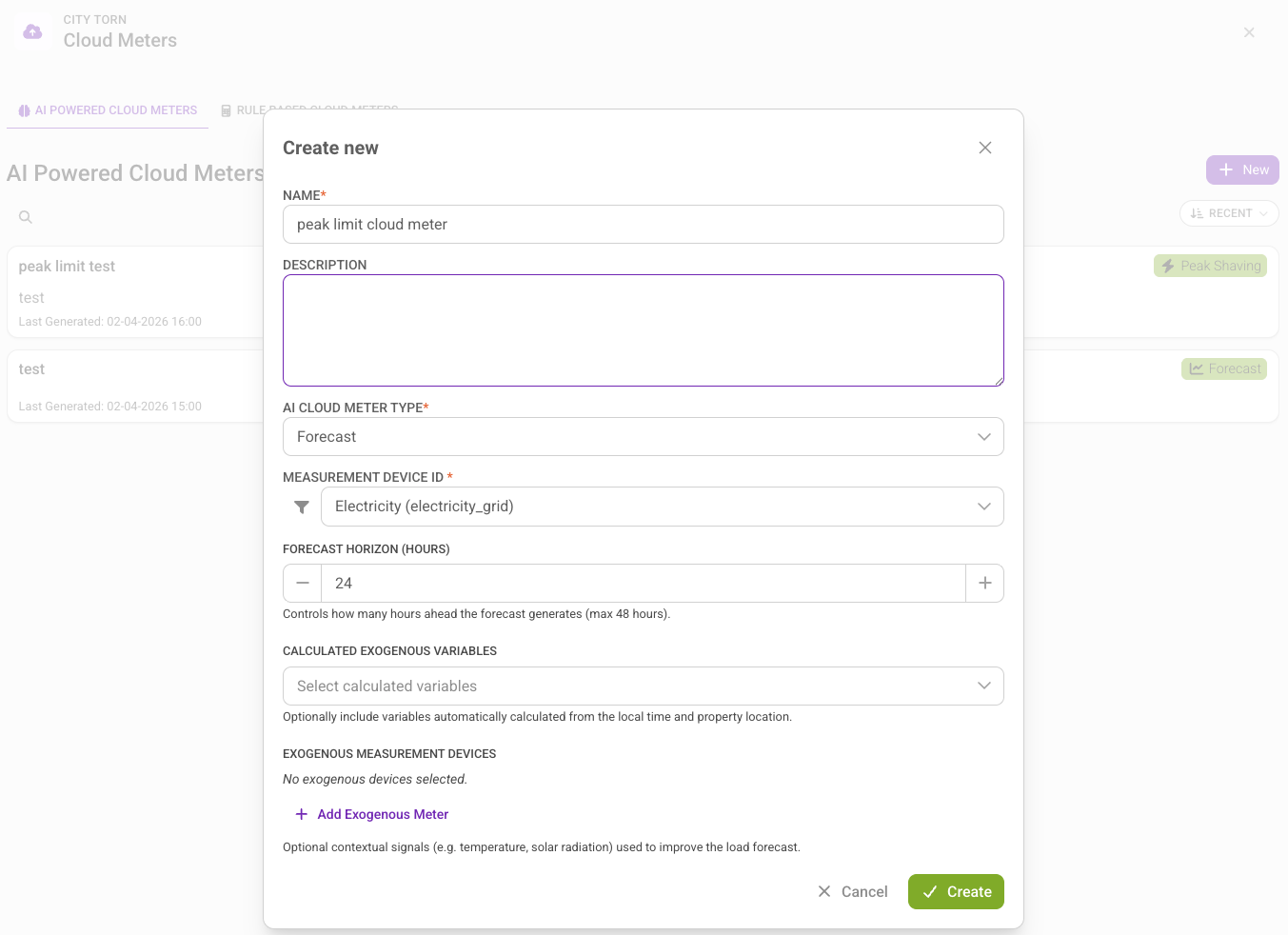
- Configure:
| Setting | Recommended starting value | Description |
|---|---|---|
| Source meter | Your grid consumption meter | Must be a grid-import consumption meter with hourly or sub-hourly intervals |
| Peak count | 3 (or match your grid operator) | Number of top peaks used for threshold calculation. Match to your billing model (single peak = 1, top-3 average = 3). |
| Reduction percent | 10% | Target reduction from historical baseline. Start conservative and tighten. |
| Forecast horizon | 24 hours | How far ahead to generate limits |
| Tariff rules | Match your grid operator contract | Define time-of-use periods and their relative price weights |
After creating the calculator, let it run for at least a few days before connecting the edge conductor. The calculator needs to build up cost factor history and stabilize the threshold. Running the conductor against unstable limits can cause unnecessary load shedding.
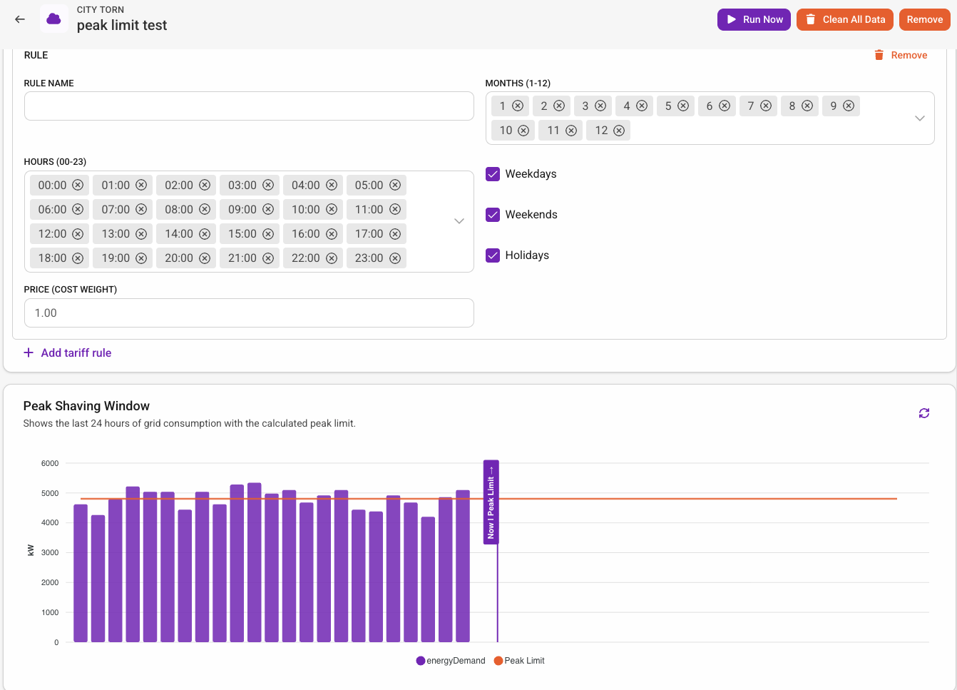
What the calculator produces
The calculator creates two output measurement devices:
- Peak Limit — Hourly kW limit values for the forecast window. This is what the edge conductor fetches and enforces.
- Cost Factor — Hourly cost factor values (kW x price weight). Useful for diagnostics.
The edge conductor polls the cloud hourly for updated limits using getPeakShavingLimits. Each limit specifies a time window (from, to) and a power value in kW. The conductor matches the current time to the active limit.
Step 4 — Configure the Peak Shaving Conductor on the edge
The conductor is a Bench node (lar-peak-shaving) that runs on the edge device. It ties everything together: reading the grid meter, fetching limits, and orchestrating load controllers.
How the conductor works
The conductor uses a two-point controller with hysteresis to make shed/recover decisions:
   SHED zone          │  Dead band  │  RECOVER zone
   ───────────────────┼─────────────┼───────────────────
              Peak Limit    Limit × Hysteresis
- When grid power exceeds the peak limit → start shedding loads (highest-priority first)
- When grid power drops below limit x hysteresis → start recovering loads (lowest-priority first, reverse order)
- When grid power is between the two thresholds (dead band) → hold current state, no action
The hysteresis dead band prevents rapid on/off oscillation. With a limit of 100 kW and hysteresis of 0.85, the conductor sheds at 100 kW and doesn't recover until power drops below 85 kW.
Node configuration
You can open the Bench editor directly from the platform: navigate to your site → Edge Devices, select the device, and click Remote Management. This gives you secure access to the device's Bench interface without needing local network access.
Open the edge device's Bench editor and add the Peak Shaving node.
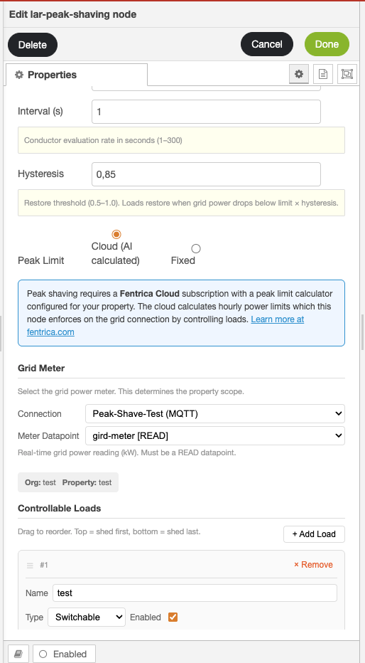
| Setting | Description |
|---|---|
| Peak Limit mode | Cloud (AI calculated) — uses limits from the Peak Shaving Calculator. Fixed — uses a constant limit (useful for testing). |
| Interval | Evaluation rate in seconds (1–300). How often the conductor reads the grid meter and makes decisions. Default: 60s. Lower values react faster but generate more control writes. |
| Hysteresis | Restore threshold ratio (0.5–1.0). Default: 0.85. Loads restore when grid power drops below limit x hysteresis. Lower values create a wider dead band (less oscillation, slower recovery). |
| Grid meter | Select the connection and datapoint for the grid power meter. This is the READ datapoint configured in Step 1. |
| Controllable loads | Add loads in priority order. Order matters — loads at the top are shed first and recovered last. |
Load priority strategy
The conductor processes loads in the order you define. Design your priority list based on:
| Priority | Shed first, recover last | Rationale |
|---|---|---|
| 1 (highest) | Battery discharge | Fastest response, no comfort impact, recovers automatically |
| 2 | Non-essential HVAC (pre-heating, ventilation boost) | Temporary comfort reduction, large kW impact |
| 3 | EV charging | Deferrable, large kW impact |
| 4 | Lighting (dimming) | Noticeable but tolerable |
| 5 (lowest) | Essential HVAC (main cooling/heating) | Last resort — comfort impact |
Priority and the shed budget
When the conductor decides to shed, it walks the list top-to-bottom, asking each load controller: "Can you shed X kW?" Each controller proposes a decision (based on its current state, timing guards, and capacity), and the conductor applies it and subtracts the freed kW from the remaining budget. It stops once the budget is exhausted or all loads are shed.
Recovery works the same way but in reverse order — bottom-to-top — so essential loads are restored first.
Reporting
Every shed and recover decision is reported to the cloud as an OPTIMIZATION_PEAK_SHAVING event with full context:
| Field | Description |
|---|---|
action | shed or recover |
loadName | Which load was affected |
loadType | switchable, curtailable, or battery |
deltaKw | How much power was freed or restored |
gridKw | Grid power at the time of the decision |
limitKw | Active peak limit at the time |
These events appear in the site's Logs and are linked to the relevant technical system, giving you a complete audit trail of every peak shaving action.
Example: office building with battery and HVAC
Consider a 500 kW office building with:
- Grid meter — Modbus TCP to the main utility meter
- 100 kWh / 50 kW battery — Modbus TCP to a Huawei inverter
- 2 x rooftop AHUs — BACnet/IP, 30 kW each, curtailable to 10 kW
- Water heater — Relay control, 15 kW, switchable
Calculator output
The Peak Shaving Calculator determines that the optimal daytime limit is 380 kW based on the top-3 billing model with a 10% reduction target.
What happens when a spike hits
~10 seconds
- 09:15:00 — Grid power spikes to 395 kW (morning startup + EV charging). The conductor detects
395 > 380(above limit). - 09:15:00 — Conductor walks the priority list. Battery controller proposes discharging 15 kW (the excess). Decision applied — battery writes -15 kW to the inverter.
- 09:15:10 — Next evaluation. Grid reads 380 kW. In the dead band (between 380 and 323 kW). Hold.
- 09:45:00 — Morning startup subsides. Grid drops to 310 kW. Below
380 x 0.85 = 323 kW. Conductor recovers the battery — writes 0 kW (idle), unlocks the datapoint.
If the spike had been larger (e.g., 420 kW), the battery alone would not be enough. The conductor would continue down the priority list: battery discharges 50 kW (max), then AHU-1 curtails from 30 kW to 20 kW (frees 10 kW). Total reduction: 60 kW → grid drops from 420 to 360 kW.
Monitoring and troubleshooting
Node status display
The conductor node shows real-time status in the Bench editor:
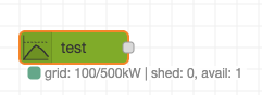
| Status | Meaning |
|---|---|
| `grid: 350/380kW | shed: 0, avail: 3` (green) |
| `grid: 375/380kW | shed: 0, avail: 3` (yellow) |
| `grid: 395/380kW | shed: 1, avail: 2` (red) |
Common issues
| Symptom | Likely cause | Fix |
|---|---|---|
| "No peak limit" error | Calculator not running or no limits generated yet | Verify the AI Cloud Meter is active and has generated limits. Check that orgId and propertyId match. |
| "Grid meter not available" | Connection or datapoint not loaded | Verify the grid meter connection is online. Check the edge device diagnostics page. |
| Loads not shedding despite grid over limit | All loads already shed, or timing guards active | Check the conductor output for limit_exceeded events. Review minOffTimeMin and cooldownPeriodMin settings. |
| Rapid on/off cycling | Hysteresis too high (dead band too narrow) or cooldownPeriodMin not set | Lower hysteresis (e.g., 0.80) to widen the dead band. Set cooldownPeriodMin on switchable loads. |
| Battery not discharging | SOC below floor | Check the SOC datapoint value. Adjust minSocPercent if the floor is too conservative. |
Best practices
- Start with Cloud limits, not Fixed — The AI calculator adapts to your building's consumption patterns and tariff structure. Fixed limits are useful for testing but miss the self-learning benefit.
- Battery first in priority — Batteries respond instantly and have no comfort impact. Use them as the first line of defense, with HVAC and other loads as backup.
- Set evaluation interval to 10–30 seconds for buildings with batteries — Batteries can absorb spikes quickly, but only if the conductor detects them quickly. For buildings with only switchable/curtailable loads, 60 seconds is fine.
- Use ramp rates on curtailable loads — Sudden setpoint changes (e.g., VFD from 30 kW to 10 kW in one step) can cause pressure or temperature shocks. A ramp rate of 5 kW per step smooths the transition.
- Monitor the first week closely — Watch the logs for shed/recover patterns. If loads are shedding and recovering too frequently, widen the hysteresis or add cooldown periods. If they never shed, the limit may be too generous — tighten the reduction target.
- Review load priority seasonally — In winter, HVAC heating is essential and should be low priority (shed last). In summer, cooling is essential. Adjust priority order with the seasons.